
SLAM_with_GTSAM
The code implements two algorithms, batch and incremental, for 2D trajectory optimization using gtsam library. The input data is obtained from a g2o file containing the 2D poses and edges between them. The batch solution uses Gauss-Newton method to optimize the graph, while the incremental solution uses iSAM2 algorithm to optimize the graph incrementally in every timestep. A prior factor model is added to the graph to improve optimization performance. The optimized trajectories are then plotted and saved as figures. The code also includes a function to convert the optimized poses from gtsam Pose2 objects to numpy arrays for easier plotting. Overall, this code provides a basic implementation for 2D trajectory optimization using gtsam library.
2-Dimentional Graph SLAM
Batch Solution
Input : file name
Output: result
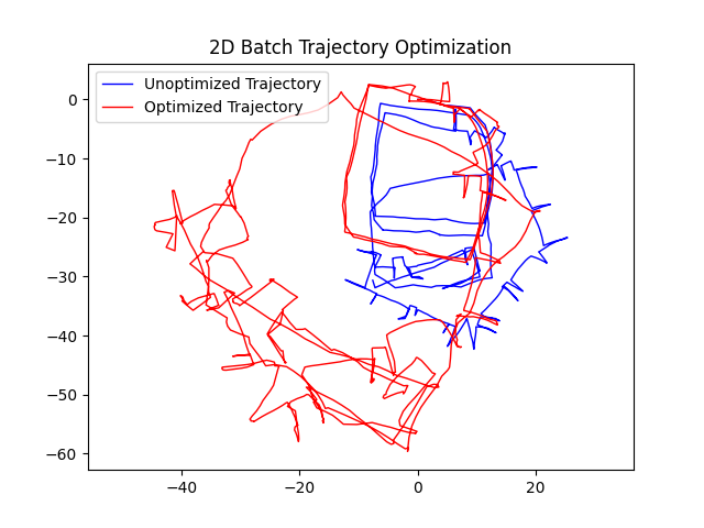
The goal is to optimize the trajectory with the batch method using the input g2o file “input_INTEL_g2o.g2o”. There are mainly five steps, which are reading the data, add a prior factor model, build a optimizer with the Gauss-Newton method, optimize the graph and initial to a gtsam.Pose2 structure, and plot the x, y position.
The predefined gtsam.readG2o(file, is3D) function phrases a G2o file and stores the measurements into a gtsam.NonlinearFactorGraph structure and the initial estimate into a gtsam.Values structure. The function set a flag ‘is3D’ to false since it’s a 2D graph.
The following step is to add a prior factor to a existing graph. We have to define a noiseModel first, build a factorPose2 with the noiseModel and add the factorPose2 to the graph. Noisemodel can be build with Diagnoal, Gaussian, Isotropic, Constrained, and Unit, and I choose the gtsam.noiseModel.Diagonal.Variances() method with specifing the variances of the 33 matrix using np.array([1e-6, 1e-6, 1e-4]). The prior factor have to be created subsequently with gtsam.PriorFactorPose2(0, gtsam.Pose2(), priorModel) to be added to the graph. Then we can add the priorFactorPose2 to the graph with measurements.
We want to solve the non-linear least square problem with the Gauss-Newton method. Thus, we give the gtsam.GaussNewtonOptimizer(graph, initial, params) function with the measurement graph with priorFactor, the initial estimate, and configuration parameters with gtsam.GaussNewtonParams(). After optimizing with the Gauss-Newton method, the gtsam.optimize() method is used for building the graph, initial to a Pose2 structure. With the Pose2 structure, I define a pose2_to_array(result) function which change the Pose2 structure to an np.array and extract the x, y values for plotting the initial and result.
Incremental Solution
Input: poses (Nx4) [i x y theta]
edges (Nx11) [i j x y theta info(x, y, theta)] Output: result
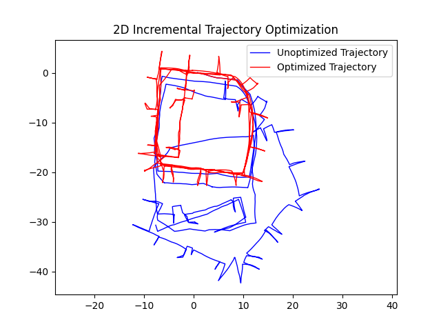
The goal is to optimize the trajectory with the incremental method using the input g2o file “input_INTEL_g2o.g2o”. There are mainly seven steps, which are reading the data, initialize ISAM2, add a prior factor model, calculate the information matrix for the moisemodel, update the isam with the current graph and initial estimate, calculate the estimate every timestep and convert to a gtsam.Pose2 structure, and plot the x, y position.
After reading the data through the readG2OFile2d(file_name) function, we can initialize the isam with gtsam.ISAM2(params) given the configuration parameters set by gtsam.ISAM2Params().
The following step is to add a prior factor to a new graph. We have to define a noiseModel first, build a factorPose2 with the noiseModel and add the factorPose2 to the graph. Noisemodel can be build with Diagnoal, Gaussian, Isotropic, Constrained, and Unit, and I choose the gtsam.noiseModel.Diagonal.Variances() method with specifing the variances of the 33 matrix using np.array([1e-6, 1e-6, 1e-4]). The x, y, theta are 0 with the 0-index and can be added to the prior factor with the Pose2 structure. The prior factor have to be created subsequently with gtsam.PriorFactorPose2(0, gtsam.Pose2(x, y, theta), priorModel) to be added to the graph. Then we can add the priorFactorPose2 to the graph, and insert the pose2(x, y, theta) to the initial_estimate.
After adding the priorFactor, we have to update the isam with isam.update(graph, initial_estimate) and calculate the estimate with calculateEstimate() which will happen in every timestep.
Starting from now, we steps will be repeated until the data in finish calculating. The previously calculated pose was inserted into the initial_estimate with the corresponding index. Detailed data including index, x, y, and data for information matrix are extracted from the edges. The noise model was build with Information matrix was build with gtsam.noiseModel.Gaussian.Covariance(cov) which cov was the inverse of the information matrix. The FactorPose2 have to be created subsequently with gtsam.BetweenFactorPose2(int(ide1), int(ide2), gtsam.Pose2(dx, dy, dtheta), model) to be added to the graph.
After the iterations, we would return the result with the Pose2 structure. The pose2_to_array(result) function would change the Pose2 structure to an np.array and extract the x, y values for plotting the initial and result.
| 2D - Batch Solution | 2D - Incremental Solution |
|---|---|
 |
 |
3-Dimentinoal Graph SLAM
Batch Solution
Input: file name
Output: result
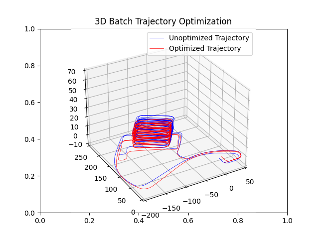
The goal is to optimize the trajectory with the batch method using the input g2o file “parking-garage.g2o”. There are mainly five steps, which are reading the data, add a prior factor model, build a optimizer with the Gauss-Newton method, optimize the graph and initial to a gtsam.Pose3 structure, and plot the x, y, z position. The steps are the same as the 3D batch solutions, but we would have a dataset with 3-dimentional measurements, which instead of Pose3 structure, we use Pose3 structure.
The predefined gtsam.readG2o(file, is3D) function phrases a G2o file and stores the measurements into a gtsam.NonlinearFactorGraph structure and the initial estimate into a gtsam.Values structure. The function set a flag ‘is3D’ to true since it’s a 3D graph.
The following step is to add a prior factor to a existing graph. We have to define a noiseModel first, build a factorPose3 with the noiseModel and add the factorPose3 to the graph. Noisemodel can be build with Diagnoal, Gaussian, Isotropic, Constrained, and Unit, and I choose the gtsam.noiseModel.Diagonal.Variances() method with specifing the variances of the 66 matrix using np.array([1e-6, 1e-6, 1e-6, 1e-4, 1e-4, 1e-4]). The prior factor have to be created subsequently with gtsam.PriorFactorPose3(0, gtsam.Pose3(), priorModel) to be added to the graph. Then we can add the priorFactorPose3 to the graph with measurements.
We want to solve the non-linear least square problem with the Gauss-Newton method. Thus, we give the gtsam.GaussNewtonOptimizer(graph, initial, params) function with the measurements graph with priorFactor, the initial estimate, and configuration parameters with gtsam.GaussNewtonParams(). After optimizing with the Gauss-Newton method, the gtsam.optimize() method is used for building the graph, initial to a Pose3 structure. With the Pose3 structure, I define a pose3_to_array(result) function which change the Pose3 structure to an np.array and extract the x, y values for plotting the initial and result.
Incremental Solition
Input: poses (Nx8) [i x y theta]
edges (Nx30) [i j x y theta info(x, y, theta)] Output: result
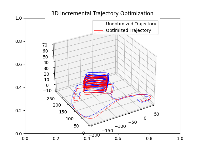
The goal is to optimize the trajectory with the incremental method using the input g2o file “parking-garage.g2o”. There are mainly seven steps, which are reading the data, initialize ISAM2, add a prior factor model, calculate the information matrix for the moisemodel, update the isam with the current graph and initial estimate, calculate the estimate every timestep and convert to a gtsam.Pose3 structure, and plot the x, y, z position.
After reading the data through the readG2OFile3d(file_name) function, we can initialize the isam with gtsam.ISAM2(params) given the configuration parameters set by gtsam.ISAM2Params().
The following step is to add a prior factor to a new graph. We have to define a noiseModel first, build a factorPose3 with the noiseModel and add the factorPose3 to the graph. Noisemodel can be build with Diagnoal, Gaussian, Isotropic, Constrained, and Unit, and I choose the gtsam.noiseModel.Diagonal.Variances() method with specifing the variances of the 66 matrix using np.array([1e-6, 1e-6, 1e-6, 1e-6, 1e-4, 1e-4]). The priorPose named prior can be calculated through the quaternion rotation matrix and transition matrix with quaternion_rotation_matrix(qw, qx, qy, qz) and np.array([x, y, z]).reshape((3, 1)) respectively. The prior factor have to be created subsequently with gtsam.PriorFactorPose3(0, prior, priorModel) to be added to the graph. Then we can add the priorFactorPose3 to the graph, and insert the pose to the initial_estimate.
After adding the priorFactor, we have to update the isam with isam.update(graph, initial_estimate) and calculate the estimate with calculateEstimate() which will happen in every timestep.
Starting from now, we steps will be repeated until the data in finish calculating. The previously calculated pose was inserted into the initial_estimate with the corresponding index. Detailed data including index, x, y, z, qx, qy, qz, qw and data for information matrix are extracted from the edges. The noise model was build with Information matrix was build with gtsam.noiseModel.Gaussian.Covariance(cov) which cov was the inverse of the information matrix. The currentPose named pose can be calculated through the quaternion rotation matrix and transition matrix with quaternion_rotation_matrix(qw, qx, qy, qz) and np.array([x, y, z]).reshape((3, 1)) respectively. The FactorPose3 have to be created subsequently with gtsam.BetweenFactorPose3(int(ide1), int(ide2), pose, model) to be added to the graph.
After the iterations, we would return the result with the Pose3 structure. The pose3_to_array(result) function would change the Pose3 structure to an np.array and extract the x, y, z values for plotting the initial and result.
| 3D - Batch Solution | 3D - Incremental Solution |
|---|---|
 |
 |